Binary Tree Traversal: Recursive and Level-Order Approaches

Once you finish this piece, you will be able to handle these LeetCode problems:

What You Need First

Before diving in, make sure you understand the basic ideas behind binary trees and a few of their special forms.

The Core Idea in One Line

Binary trees can be walked in exactly two styles: recursive traversal and level-order traversal. That is the complete picture. Recursive traversal is the foundation of depth-first search (DFS), while level-order traversal is the foundation of breadth-first search (BFS).

Recursive traversal always follows one fixed path through the nodes, yet it offers three distinct moments where you can place your own code, and each moment produces a different result. Level-order traversal likewise follows a fixed node order, but it can be written in three different styles, each useful for particular kinds of problems.

Recursive Traversal (DFS)

Here is the basic skeleton for recursive traversal of a binary tree:

# fundamental binary-tree node
class TreeNode:
    def __init__(self, val=0, left=None, right=None):
        self.val = val
        self.left = left
        self.right = right

# skeleton for recursive binary-tree traversal
def traverse(root: TreeNode):
    if root is None:
        return
    traverse(root.left)
    traverse(root.right)

How can such a short function visit every node of a binary tree, and in what sequence does it do so?

You can picture the recursive function as a pointer that moves around the tree. The video that follows shows exactly how that pointer travels.

The code itself says the same thing: it calls itself on root.left before it ever calls itself on root.right. Every entry into traverse therefore explores the left child first; the right child receives attention only after a null pointer stops further leftward progress.

Making Sense of Preorder, Inorder, and Postorder

The order in which the traverse function itself visits nodes is indeed fixed. The video always shows the root pointer moving through the tree in the same path.

Nevertheless, statements placed at different locations inside the traverse function produce different observable effects. Preorder, inorder, and postorder traversals yield different results simply because their code occupies different spots.

When you first arrive at a node you still know nothing about its children. When you are about to leave a node you have already finished both of its subtrees. Code executed at those two different moments can therefore behave differently.

Preorder, inorder, and postorder traversal are really just names for the three places you may insert code inside the binary-tree traversal skeleton:

# Binary-tree traversal skeleton
def traverse(root):
    if root is None:
        return
    # Pre-order position
    traverse(root.left)
    # In-order position
    traverse(root.right)
    # Post-order position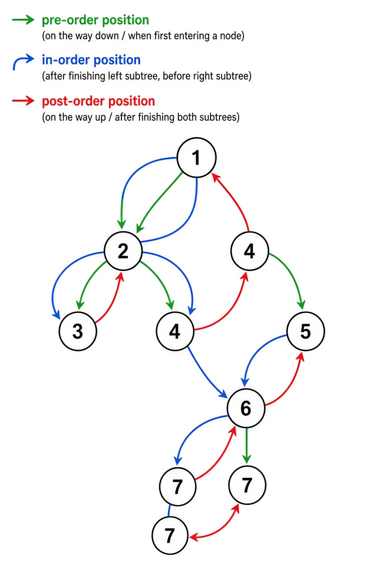

Code in the preorder position runs the instant you enter a node; code in the inorder position runs after the left subtree has finished and before the right subtree begins; code in the postorder position runs only after both the left and the right subtrees have been completely processed.

Level-Order Traversal (BFS)

Level-Order Traversal (BFS)

The recursive approach we examined earlier depends on the call stack to walk the tree. It begins at the leftmost leaf and advances column by column until it reaches the rightmost side.

Level-order traversal, by contrast, processes the tree one horizontal layer at a time, moving from left to right within each layer.

This style of traversal is built around a queue. Depending on the information you need, there are three common ways to write it. We will look at each one in turn.

Version 1

This is the most straightforward form. The code looks like this:

from collections import deque

def levelOrderTraverse(root):
    if root is None:
        return
    q = deque()
    q.append(root)
    while q:
        cur = q.popleft()
        # process the current node
        print(cur.val)

        # enqueue the left and right children if they exist
        if cur.left is not None:
            q.append(cur.left)
        if cur.right is not None:
            q.append(cur.right)

In the below video, you will see that the cur pointer visits nodes layer by layer, always left to right within a layer.

Strengths and Weaknesses of This Version

Its main benefit is simplicity. You repeatedly remove the node at the front of the queue and immediately enqueue its children. Nothing more is required.

The drawback is that you have no way to know which layer the current node belongs to. Many problems need that information—for example, when you must gather every node on a given layer or compute the minimum depth of the tree.

Because of this limitation, the simple version is rarely used in practice. The next version is far more common.

Version 2

A small change to the previous approach produces the following version:

from collections import deque

def levelOrderTraverse(root):
    if root is None:
        return

    q = deque()
    q.append(root)

    # track the layer currently being processed (root starts at layer 1)
    depth = 1

    while q:
        sz = len(q)
        for i in range(sz):
            cur = q.popleft()
            # process the current node together with its layer
            print(f"depth = {depth}, val = {cur.val}")

            # enqueue the left and right children if they exist
            if cur.left is not None:
                q.append(cur.left)
            if cur.right is not None:
                q.append(cur.right)
        depth += 1

Pay attention to the inner loop:

sz = len(q)
for i in range(sz):
    ...

The variable i simply counts the position of the current node inside the present layer. Most problems never need that count, so an equivalent form is:

sz = len(q)
while sz > 0:
    ...
    sz -= 1

Either style is fine.

One important detail: you must capture the queue length in sz before the loop begins. The queue grows as children are added, so you cannot use len(q) directly as the loop condition.

In the video the visit order remains layer by layer from left to right, but each node is now accompanied by its layer number.

Because this version records the layer of every node, it can solve problems such as finding the minimum depth of a binary tree. It is the form of level-order traversal used most often.

Version 3

If version 2 already covers the majority of cases, why introduce a third version? It prepares the ground for more advanced algorithms that appear later.

At the moment we are only discussing binary trees, yet the same idea extends to N-ary trees, graph BFS, and the general BFS enumeration framework. It is therefore useful to widen the perspective here.

In version 2 we simply increment a single depth counter each time we finish a layer. You can view every edge as having weight 1, so the depth of a node is exactly the sum of the edge weights along the path from the root. All nodes on the same layer share the same path-weight sum.

Now imagine that edges may carry arbitrary weights and you are asked to visit the tree layer by layer while printing each node’s path-weight sum. How would you proceed?

In that setting nodes on the same layer no longer share a single common sum, so a lone depth variable is no longer sufficient.

Version 3 solves precisely this problem. It starts from the simple queue of version 1 and attaches a small State object to every entry so that each node carries its own path-weight sum. The code is:

class State:
    def __init__(self, node, depth):
        self.node = node
        self.depth = depth

def levelOrderTraverse(root):
    if root is None:
        return
    q = deque()
    # the path weight sum of the root is 1
    q.append(State(root, 1))

    while q:
        cur = q.popleft()
        # process the current node together with its path weight sum
        print(f"depth = {cur.depth}, val = {cur.node.val}")

        # enqueue the left and right children, each carrying an updated sum
        if cur.node.left is not None:
            q.append(State(cur.node.left, cur.depth + 1))
        if cur.node.right is not None:
            q.append(State(cur.node.right, cur.depth + 1))

Open the visualization panel and step through it. Nodes are still visited layer by layer from left to right, and each node’s path-weight sum is printed.

In this design every node is responsible for its own depth (or path-weight sum). The approach is the most flexible of the three and can meet the needs of any BFS algorithm. Creating an extra State class does add a little overhead, however, so version 2 remains preferable unless the extra flexibility is required.

As you will see later, weighted edges belong to the domain of graph algorithms. You will not need version 3 until the later BFS exercises and the Dijkstra algorithm.