Circular Arrays: Concept and Code

What You Should Know First
You will get more out of this explanation if you already understand how ordinary arrays store elements in consecutive memory locations.

Quick Overview
A circular array applies the modulo (remainder) operator so that a plain linear array behaves as if its ends are joined. This arrangement makes it possible to insert or delete an element at the front in (O(1)) time.

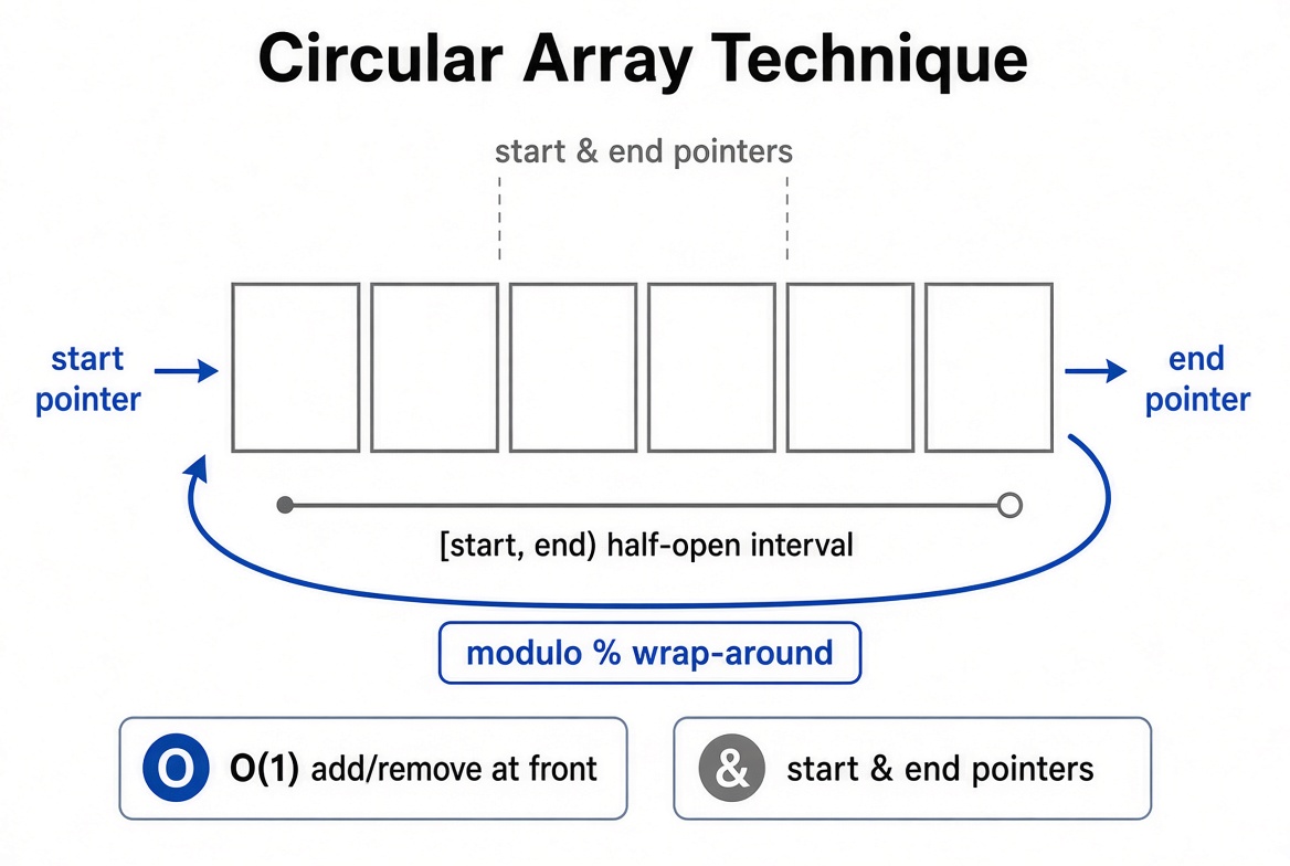
Making an Array Behave Circularly
An array cannot literally form a circle; it occupies a single contiguous stretch of memory. We can still treat it as circular for the purpose of indexing. The short program below demonstrates the idea:

# length-5 array
arr = [1, 2, 3, 4, 5]
i = 0
# endless traversal that wraps around
while i < len(arr):
    print(arr[i])
    i = (i + 1) % len(arr)

The decisive step is the expression (i + 1) % len(arr). As soon as the index reaches the final position, the remainder calculation forces it back to zero, returning us to the first element. The loop therefore continues forever, producing the logical effect of a circle.

That wrapping behavior is the essence of the circular-array technique. It is also what permits front-end insertion and deletion in constant time.

Consider a capacity-6 array that currently holds three values (blank slots shown as _):

[1, 2, 3, _, _, _]

Removing the front value can be performed simply by marking its slot empty:

[_, 2, 3, _, _, _]

No other elements need to move. If we next insert 4 and then 5 at the front, the second insertion has nowhere to go on the left side, so it wraps around and lands at the opposite end:

[4, 2, 3, _, _, 5]

The Essential Mechanism
The picture above is only an illustration. In a working implementation we maintain two indices, conventionally called start and end.

start always identifies the position of the first live element.

end always identifies the position immediately after the last live element.

Consequently, every front-end operation reduces to a single adjustment of start, and every back-end operation reduces to a single adjustment of end. Whenever either index would step outside the legal range (< 0 or >= capacity), the modulo operator folds it back to the opposite end. The net result is a circular buffer.

Interactive Exploration
Reading the description is useful, yet the clearest understanding comes from watching the pointers move. The visualization pane contains a live circular array. Click arr.addLast or arr.addFirst and observe how start, end, and the stored values change together.

Implementation Details

Interval Convention
The code treats the occupied region as a half-open interval [start, end). Every other method is written against that convention.

Why prefer a left-closed, right-open interval? With the initial state start = end = 0 the interval [0, 0) is empty. Advancing end by one step produces [0, 1), which contains exactly the element at index 0.

A fully open interval would still be empty after the same move, while a fully closed interval would already contain an element at initialization. Both alternatives force awkward special-case handling; the half-open form avoids them.

The complete implementation follows:

class CycleArray:
    def __init__(self, size=1):
        self.size = size
        # Python lists can hold any objects, so no extra conversion is required
        self.arr = [None] * size
        # start indexes the first occupied slot (inclusive)
        self.start = 0
        # end indexes one past the last occupied slot (exclusive)
        self.end = 0
        self.count = 0

    # grow or shrink the underlying storage
    def resize(self, newSize):
        # allocate fresh storage
        new_arr = [None] * newSize
        # transfer existing elements in logical order
        for i in range(self.count):
            new_arr[i] = self.arr[(self.start + i) % self.size]
        self.arr = new_arr
        # re-anchor the two pointers
        self.start = 0
        self.end = self.count
        self.size = newSize

    # insert at the front, O(1)
    def add_first(self, val):
        # double capacity when full
        if self.is_full():
            self.resize(self.size * 2)
        # move start left, then write (because start is inclusive)
        self.start = (self.start - 1 + self.size) % self.size
        self.arr[self.start] = val
        self.count += 1

    # delete from the front, O(1)
    def remove_first(self):
        if self.is_empty():
            raise Exception("Array is empty")
        # read, clear, then advance start
        val = self.arr[self.start]
        self.arr[self.start] = None
        self.start = (self.start + 1) % self.size
        self.count -= 1
        # shrink when occupancy drops to one-quarter
        if self.count > 0 and self.count == self.size // 4:
            self.resize(self.size // 2)
        return val

    # insert at the back, O(1)
    def add_last(self, val):
        if self.is_full():
            self.resize(self.size * 2)
        # write, then advance end (because end is exclusive)
        self.arr[self.end] = val
        self.end = (self.end + 1) % self.size
        self.count += 1

    # delete from the back, O(1)
    def remove_last(self):
        if self.is_empty():
            raise Exception("Array is empty")
        # retreat end, then read and clear
        self.end = (self.end - 1 + self.size) % self.size
        val = self.arr[self.end]
        self.arr[self.end] = None
        self.count -= 1
        # shrink when occupancy drops to one-quarter
        if self.count > 0 and self.count == self.size // 4:
            self.resize(self.size // 2)
        return val

    # peek at the front element, O(1)
    def get_first(self):
        if self.is_empty():
            raise Exception("Array is empty")
        return self.arr[self.start]

    # peek at the back element, O(1)
    def get_last(self):
        if self.is_empty():
            raise Exception("Array is empty")
        # end is exclusive, so the last live index is one step earlier
        return self.arr[(self.end - 1 + self.size) % self.size]

    def is_full(self):
        return self.count == self.size

    def size(self):
        return self.count

    def is_empty(self):
        return self.count == 0

Further Reflection
Must insertion or deletion at the front of an array always cost linear time?
In a conventional array the answer is yes, because every element after the insertion or deletion point must be shifted. A circular array removes that necessity: both front-end operations become constant-time.

The class shown above supplies only the four end-point operations (add_first, remove_first, add_last, remove_last). Earlier dynamic-array discussions also included index-based insertion, deletion, and random access. Those operations remain feasible with a circular layout, and their asymptotic costs do not worsen:

Deleting an arbitrary index still requires shifting the intervening elements, so the cost stays (O(n)).

Reading an arbitrary index is still (O(1)); the only extra work is a constant-time offset calculation from start.

Inserting at an arbitrary index likewise requires shifting, remaining (O(n)).

The reasoning appears sound. That raises a natural question: why do the dynamic-array containers supplied by most language standard libraries not adopt the circular-array technique internally?